Thursday, September 30, 2010

Multiview Video Coding - 01


Multiview Video Coding

Introduction:

The need for multiview video coding is driven by two recent technological developments: new 3D video/display technologies and the growing use of multi-camera arrays. A variety of companies are starting to produce 3D displays that do not require glasses and can be viewed by multiple people simultaneously. The immersive experience provided by these 3D displays are compelling and have the potential to create a growing market for 3D video and hence for multiview video compression. Furthermore, even with 2D displays, multi-camera arrays are increasingly being used to capture a scene from many angles. The resulting multiview data sets allow the viewer to observe a scene from any viewpoint and serve as another application of multiview video compression.

In July 2008, MPEG officially approved an amendment of the ITU-T Rec. H.264 & ISO/IEC 14996-10 Advanced Video Coding (AVC) standard on Multiview Video Coding. MVC is an extension of the AVC/H.264 standard that provides efficient encoding or compressed representation of sequences captured simultaneously from multiple cameras by exploiting correlation among neighboring camera views. MVC is intended for encoding stereoscopic (two-view) video, as well as free viewpoint television and multi-view 3D television applications. The Stereo High profile has been standardized in June 2009; the profile is based on MVC toolset and is used in stereoscopic Blu-ray 3D releases.

MVC stream is backward compatible with H.264/AVC, which allows older devices and software to decode stereoscopic video streams, ignoring additional information for the second view. 3D video (3DV) and free viewpoint video (FVV) are new types of visual media that expand the user's experience beyond what is offered by 2D video. 3DV offers a 3D depth impression of the observed scenery, while FVV allows for an interactive selection of viewpoint and direction within a certain operating range.  A common element of 3DV and FVV systems is the use of multiple views of the same scene that are transmitted to the user.
The overall structure of MVC defining the interfaces is illustrated in the figure below. The encoder receives N temporally synchronized video streams and generates one bitstream. The decoder receives the bitstream, decodes and outputs the N video signals.

Fig 1: Multiview Video Coding (MVC)

Multiview video contains a large amount of inter-view statistical dependencies, since all cameras capture the same scene from different viewpoints. Therefore, combined temporal and inter-view prediction is the key for efficient MVC. As illustrated in the figure below a picture of a certain camera can not only be predicted from temporally related pictures of the same camera. Also pictures of neighboring cameras can be used for efficient prediction.

Fig 2: Temporal/inter-view prediction structure for MVC

Application Areas:
  • Stereo Scope Video
  • 3D Video/Display
  • Free Viewpoint Video
Topics Related to MVC:
  • Multiview Coding Structures
  • Multiview Coding Tools
  • Inter-view Prediction
  • Illumination Compensation
  • Disparity, Depth and 3D Geometry Coding
  • View Interpolation Prediction
  • Scene Analysis and View Synthesis
  • Random Access Aspects in MVC
  • Multiview Communication Systems
  • Multiview Coding Applications
  • Performance and Complexity Issues in MVC

.

Wednesday, September 29, 2010

Post a Video to Blog from YouTube

How do I post a video to my blog from YouTube?

If you've got your own videos on your computer that you want to share on your blog, Blogger now allows you to upload video directly!


If you'd like to share a video from YouTube, you can do that, too.

Embedding a YouTube Video

To embed a video from YouTube, just copy the code from the "Embed" box on the video's YouTube page. You can find the "Embed" box in the "About This Video" box when you're watching the video. You can also get the code from the "Embed HTML" box on the "Edit Video" page if the video belongs to your YouTube account. Or simply right click on the video and copy the "embedded html code".


To embed a YouTube video within a blog post, first click "Edit HTML" from within the post editor. Next, paste the video's code into the body of your post. That's it!

Set Up One-Click Video Sharing

If you post YouTube videos to your blog regularly, sharing directly from YouTube is even easier and you'll only have to set it up once.


  1. Click the "Share" button on the YouTube video's page
  2. Scroll down and click "Setup your blog for video posting."
  3. Click "Add a Blog/Site"
  4. Choose "Blogger" as your Blog Service and fill in your Google Account login information.
  5. Choose which blogs you'd like to add to your YouTube account. You can choose more than one.
  6. From now on, when you click "Share", you'll be given the option to post YouTube videos directly to your blogs!


Language Setting on youtube.com

In the main of youtube page (www.youtube.com)
click the "भाषा" at the bottom of the page, this will show you available languages...


Sunday, September 26, 2010

H.264 – Inter Prediction


H.264 Video Codec - Inter Prediction

Inter prediction is to reduce the temporal correlation with help of motion estimation and compensation. In H.264, the current picture can be partitioned into the macroblocks or the Submacroblock. In addition to the intra macroblock coding types, various predictive or motion-compensated coding types are allowed in P slices. Each P-type macroblock is partitioned into fixed size blocks used for motion description. Partitionings with luma block sizes of 16 × 16, 16 × 8, 8 × 16, and 8 × 8 samples are supported by the syntax. When the macroblock is partitioned into four so-called sub-macroblocks each of size 8 × 8 luma samples, one additional syntax element is transmitted for each 8 × 8 sub-macroblock. This syntax element specifies whether the corresponding sub-macroblock is coded using motion-compensated prediction with luma block sizes of 8 × 8, 8 × 4, 4 × 8, or 4 × 4 samples. Figure 1 illustrates the partitioning. The prediction signal for each predictivecoded M × N luma block is obtained by displacing a corresponding area of a previously decoded reference picture, where the displacement is specified by a translational motion vector and a picture reference index. Thus, if the macroblock is coded using four 8 × 8 sub-macroblocks, and each sub-macroblock is coded using four 4 × 4 luma blocks, a maximum of 16 motion vectors may be transmitted for a single P-slice macroblock.A macroblock of 16X16 luma samples can be partitioned into smaller block sizes up to 4X4.

Figure 1: Portioning of Macroblock an Submacroblock for Inter Prediction

The smaller block size requires larger number of bits to signal the motion vectors and extra data of the type of partition, however the motion compensated residual data can be reduced. Therefore, the choice of partition size depends on the input video characteristics. In general, a large partition size is appropriate for homogeneous areas of the frame and a small partition size may be beneficial for detailed areas. In former standards as MPEG-4 or H.263, only blocks of the size 16×16 and 8×8 are supported. The inter prediction process can form segmentations for motion representation as small as 4X4 luma samples in size, using motion vector accuracy of one-quarter of the luma sample.
A displacement vector is estimated and transmitted for each block, refers to the corresponding position of its image signal in an already transmitted reference image. In former MPEG standards this reference image is the most recent preceding image. In H.264/AVC it is possible to refer to several preceding images. This technique is denoted as motion-compensated prediction with multiple reference frames. For multi-frame motion-compensated prediction, the encoder stores decoded reference pictures in a multi-picture buffer. The decoder replicates the multi-picture buffer of the encoder according to the reference picture buffering type and memory management control operations (MMCO) specified in the bitstream. Unless the size of the multi-picture buffer is set to one picture, the index at which the reference picture is located inside the multi-picture buffer has to be signaled. For this purpose, an additional picture reference index parameter has to be transmitted together with each motion vector of 16 × 16, 16 × 8, or 8 × 16 macroblock partition or 8 × 8 submacroblock.
The process for inter prediction of a sample block can also involve the selection of the pictures to be used as the reference pictures from a number of stored previously-decoded pictures. Reference pictures for motion compensation are stored in the picture buffer. With respect to the current picture, the pictures before and after the current picture, in the display order are stored into the picture buffer. These are classified as 'short-term' and 'long-term' reference pictures. Long-term reference pictures are introduced to extend the motion search range by using multiple decoded pictures, instead of using just one decoded short-term picture. Memory management is required to take care of marking some stored pictures as 'unused' and deciding which pictures to delete from the buffer for efficient memory management.

Sub-pixel Motion Vector:
The motion vector precision is at the granularity of one quarter of the distance between luma samples. If the motion vector points to an integer-sample position, the prediction signal is formed by the corresponding samples of the reference picture; otherwise, the prediction signal is obtained using interpolation between integer-sample positions. Sub-pel motion compensation can provide significantly better compression performance than integer-pel compensation, at the expense of increased complexity. Quarter-pel accuracy outperforms half-pel accuracy. Especially, sub-pel accuracy would increase the coding efficiency at high bitrates and high video resolutions. In the luma component, the sub-pel samples at half-pel positions are generated first and are interpolated from neighboring integer-pel samples using a one-dimensional 6-tap FIR filter with weights (1, -5, 20, 20, -5, 1)/32, horizontally and/or vertically, which was designed to reduce aliasing components that deteriorate the interpolation and the motion compensated prediction. Once all the half-pel samples are available, each quarter-pel sample is produced using bilinear interpolation (horizontally, vertically, or diagonally) between neighboring half- or integer-pel samples. For 4:2:0 video source sampling, 1/8 pel samples are required in the chroma components (depending on the chroma format, corresponding to 1/4 pel samples in the luma). These samples are interpolated (linear interpolation) between integer-pel chroma samples. Sub-pel motion vectors are encoded differentially with respect to predicted values formed from nearby encoded motion vectors. After interpolation, block-based motion compensation is applied. As noted, however, a variety of block sizes can be considered, and a motion estimation scheme that optimizes the trade-off between the number of bits necessary to represent the video and the fidelity of the result is desirable.

Figure 2: Example of Integer and Sub-Pel Prediction

Skipped Mode:
In addition to the macroblock modes described above, a P-slice macroblock can also be coded in the so-called skip mode. If a macroblock has motion characteristics that allow its motion to be effectively predicted from the motion of neighboring macroblocks, and it contains no non-zero quantized transform coefficients, then it is flagged as skipped. For this mode, neither a quantized prediction error signal nor a motion vector or reference index parameter are transmitted. The reconstructed signal is computed in a manner similar to the prediction of a macroblock with partition size 16 × 16 and fixed reference picture index equal to 0. In contrast to previous video coding standards, the motion vector used for reconstructing a skipped macroblock is inferred from motion properties of neighboring macroblocks rather than being inferred as zero (i.e., no motion).

Weighted Prediction:
In addition to the use of motion compensation and reference picture selection for prediction of the current picture content, weighted prediction can be used in P slices. When weighted prediction is used, customized weights can be applied as a scaling and offset to the motion-compensated prediction value prior to its use as a predictor for the current picture samples. Weighted prediction can be especially effective for such phenomena as "fade-in" and "fade-out" scenes.

Motion Vector Prediction:
After the temporal prediction, the steps of transform, quantization, scanning, and entropy coding are conceptually the same as those for I-slices for the coding of residual data (the original minus the predicted pixel values). The motion vectors and reference picture indexes representing the estimated motion are also compressed. Because, Encoding a motion vector for each partition can take a significant number of bits, especially if small partition sizes are chosen. Motion vectors for neighbouring partitions are often highly correlated and so each motion vector is predicted from vectors of nearby, previously coded partitions. A predicted vector, MVp, is formed based on previously calculated motion vectors. MVD, the difference between the current vector and the predicted vector, is encoded and transmitted. The method of forming the prediction MVp depends on the motion compensation partition size and on the availability of nearby vectors. The "basic" predictor is the median of the motion vectors of the macroblock partitions or subpartitions immediately above, diagonally above and to the right, and immediately left of the current partition or sub-partition. The predictor is modified if (a) 16x8 or 8x16 partitions are chosen and/or (b) if some of the neighbouring partitions are not available as predictors. If the current macroblock is skipped (not transmitted), a predicted vector is generated as if the MB was coded in 16x16 partition mode.
At the decoder, the predicted vector MVp is formed in the same way and added to the decoded vector difference MVD. In the case of a skipped macroblock, there is no decoded vector and so a motioncompensated macroblock is produced according to the magnitude of MVp.

Figure 3: Multiframe Motion Compensation, I addition to the motionvector picture reference parameter also transmit.


Saturday, September 25, 2010

H.264 – Deblocking Filter


H.264 Video Codec – Deblocking Filter

This filter is also called Loopfilter, In-loop Filter, Reconstruction Filter, Adaptive Deblocking Filter and Post Filter.
Due to coarse quantization at low bit rates and block-based transformation, motion compensation, typically results in visually noticeable discontinuities along the block boundaries, as in Figure 1. If no further provision is made to deal with this, these artificial discontinuities may also diffuse into the interior of blocks by means of the motion-compensated prediction process. The removal of such blocking artifacts can provide a substantial improvement in perceptual quality.

Figure 1: Reconstructed block without Deblocking Filter

H.261 has suggested similar deblocking filter (optional) which was beneficial to reduce the temporal propagation of coded noise because only integer-pel accuracy motion compensation did not play the role for its reduction. However, MPEG-1, 2 did not use the deblocking filter because of high implementation complexity, on the other hand, the blocking artifacts can be reduced by utilizing the half-pel accuracy MC. The half-pels obtained by bilinear filtering of neighboring integer-pels played the role of the smoothing of the coded noise in the integer-pel domain.
Deblocking can in principle be carried out as post-filtering, influencing only the pictures to be displayed. Higher visual quality can be achieved though, when the filtering process is carried out in the coding loop, because then all involved past reference frames used for motion compensation will be the filtered versions of the reconstructed frames. Another reason to make deblocking a mandatory in-loop tool (in-loop filter) in H.264/AVC is to enforce a decoder to approximately deliver a quality to the customer, which was intended by the producer and not leaving this basic picture enhancement tool to the optional good will of the decoder manufacturer.
H.264 uses the deblocking filter for higher coding performance in spite of implementation complexity. Filtering is applied to horizontal or vertical edges of 4 x 4 blocks in a macroblock, as in Figure 2. The luma deblocking filter process is performed on four 16-sample edges and the deblocking filter process for each chroma components is performed on two 8-sample edges.

Figure 2: Horizontal and Vertical Edges of 4 x 4 Blocks in a Macroblock

The filtering process exhibits a high degree of content adaptivity on different levels (adaptive deblocking filter), by adjusting its strength depending upon compression mode of a macroblock (Intra or Inter), the quantization parameter, motion vector, frame or field coding decision and the pixel values. All involved thresholds are quantizer dependent, because blocking artifacts will always become more severe when quantization gets coarse. When the quantization step size is decreased, the effect of the filter is reduced, and when the quantization step size is very small, the filter is shut off. The filter can also be shutoff explicitly or adjusted in overall strength by an encoder at the slice level. As a result, the blockiness is reduced without much affecting the sharpness of the content. Consequently, the subjective quality is significantly improved. At the same time, the filter reduces bit rate by typically 5–10 percent while producing the same objective quality as the non-filtered video.

H.264/MPEG-4 AVC deblocking is adaptive on three levels:
On slice level, the global filtering strength can be adjusted to the individual characteristics of the video sequence.
On block edge level, the filtering strength is made dependent on inter/intra prediction decision, motion differences, and the presence of coded residuals in the two participating blocks. From these variables a filtering-strength parameter is calculated, which can take values from 0 to 4 causing modes from no filtering to very strong filtering of the involved block edge. Special strong filtering is applied for macroblocks with very flat characteristics to remove 'tilting artifacts'.
On sample level, sample values and quantizer-dependent thresholds can turn off filtering for each individual sample. It is crucially important to be able to distinguish between true edges in the image and those created by the quantization of the transform-coefficients. True edges should be left unfiltered as much as possible. In order to separate the two cases, the sample values across every edge are analyzed.

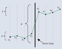
Figure 3: Sample Values inside 2 neighboring 4×4 blocks

For an explanation denote the sample values inside two neighboring 4×4 blocks as p3, p2, p1, p0 | q0, q1, q2, q3 with the actual boundary between p0 and q0 as shown in Figure 3. Filtering of the two pixels p0 and q0 only takes place, if their absolute difference falls below a certain threshold α. At the same time, absolute pixel differences on each side of the edge (|p1 − p0| and |q1 − q0|) have to fall below another threshold β, which is considerably smaller than α. To enable filtering of p1(q1), additionally the absolute difference between p0 and p2 (q0 and q2) has to be smaller than β. The dependency of α and β on the quantizer, links the strength of filtering to the general quality of the reconstructed picture prior to filtering. For small quantizer values the thresholds both become zero, and filtering is effectively turned off altogether.


 All filters can be calculated without multiplications or divisions to minimize the processor load involved in filtering. Only additions and shifts are needed. If filtering is turned on for p0, the impulse response of the involved filter would in principle be (0, 1, 4, | 4, −1, 0) / 8. For p1
it would be (4, 0, 2, | 2, 0, 0) / 8. The term in principle means that the maximum changes allowed for p0 and p1 (q0 and q1) are clipped to relatively small quantizer dependent values, reducing the low pass characteristic of the filter in a nonlinear manner.
Intra coding in H.264/AVC tends to use INTRA_16×16 prediction modes when coding nearly uniform image areas. This causes small amplitude blocking artifacts at the macro block boundaries which are perceived as abrupt steps in these cases. To compensate the resulting tiling artifacts, very strong low pass filtering is applied on boundaries between two macro blocks with smooth image content. This special filter also involves pixels p3 and q3.

Boundary strength
The choice of filtering outcome depends on the boundary strength and on the gradient of image samples across the boundary. The boundary strength parameter Bs is chosen according to the following rules:
p or q is intra coded and boundary is a macroblock boundaryBs=4 (strongest filtering)
p or q is intra coded and boundary is not a macroblock boundaryBs=3
neither p or q is intra coded; p or q contain coded coefficientsBs=2
neither p or q is intra coded; neither p or q contain coded coefficients; p and q have different referenc e frames or a different number of reference frames or different motion vector valuesBs=1
neither p or q is intra coded; neither p or q contain coded coefficients; p and q have same reference frame and identical motion vectorsBs=0 (no filtering)

The filter is "stronger" at places where there is likely to be significant blocking distortion, such as the boundary of an intra coded macroblock or a boundary between blocks that contain coded coefficients.

Filter decision
A group of samples from the set (p2,p1,p0,q0,q1,q2) is filtered only if:
(a) Bs > 0 and
(b) |p0-q0|, |p1-p0| and |q1-q0| are each less than a threshold α or β [α = (p2 – p0) and β = (q2 - q0)].
The thresholds α and β increase with the average quantizer parameter QP of the two blocks p and q. The purpose of the filter decision is to "switch off" the filter when there is a significant change (gradient) across the block boundary in the original image. The definition of a significant change depends on QP. When QP is small, anything other than a very small gradient across the boundary is likely to be due to image features (rather than blocking effects) that should be preserved and so the thresholds α and β are low. When QP is larger, blocking distortion is likely to be more significant and α, β are higher so that more filtering takes place.

Filtering process for edges with Bs
(a) Bs < 4 {1,2,3}:
A 4-tap linear filter is applied with inputs p1, p0, q0 and q1, producing filtered outputs P0 and Q0 (0<Bs<4).
In addition, if |p2-p0| is less than threshold α, a 4-tap linear filter is applied with inputs p2, p1, p0 and q0, producing filtered output P1. If |q2-q0| is less than threshold β, a 4-tap linear filter is applied with inputs q2, q1, q0 and p0, producing filtered output Q1. (p1 and q1 are never filtered for chroma, only for luma data).
(b) Bs = 4:
If |p2-p0| < β and |p0-q0| < round(α /4):
P0 is produced by 5-tap filtering of p2, p1, p0, q0 and q1
P1 is produced by 4-tap filtering of p2, p1, p0 and q0
(Luma only) P2 is produced by 5-tap filtering of p3, p2, p1, p0 and q0.
else:
P0 is produced by 3-tap filtering of p1, p0 and q1.
If |q2-q0| < α and |p0-q0| < round(β /4):
Q0 is produced by 5-tap filtering of q2, q1, q0, p0 and p1
Q1 is produced by 4-tap filtering of q2, q1, q0 and p0
(Luma only) Q2 is produced by 5-tap filtering of q3, q2, q1, q0 and p0.
else:
Q0 is produced by 3-tap filtering of q1, q0 and p1.

Settings Summary:
This setting controls most important features in Inloop Deblocking filter. In contrast to MPEG-4, the Inloop Deblocking is a mandatory feature of the H.264 standard. So the encoder, x264 in this case, can rely on the decoder to perform a proper deblocking. Furthermore all P- and B-Frames in H.264 streams refer to the deblocked frames instead of the unprocessed ones, which improves the compressibility. There is absolutely no reason the completely disable the Inloop Deblocking, so it's highly recommended to keep it enabled in all cases. There are two settings available to configure the Inloop Deblocking filter:
Strength: This setting is also called "Alpha Deblocking". It controls how much the Deblocking filter will smooth the video, so it has an important effect on the overall sharpness of your video. The default value is 0 and should be enough to smooth out all the blocks from your video, especially in Quantizer Modes (QP or CRF). Negative values will give a more sharp video, but they will also increases the danger of visible block artifacts! In contrast positivevalues will result in a smoother video, but they will also remove more details.
Threshold: This setting is also called "Beta Deblocking" and it's more difficult to handle than Alpha Deblocking. It controls the threshold for block detection. The default value is 0 and should be enough to detect all blocks in your video. Negative values will "save" more details, but more blocks might slip through (especially in flat areas). In contrast positive values will remove more details and catch more blocks.
Remarks: Generally there is no need to change the default setting of 0:0 for Strength:Threshold, as it gives very good results for a wide range of videos. Nevertheless you can try out different settings to find the optimal settings for your eyes. If you like a more sharp video and don't mind a few blocks here and there, then you might be happy with -2:-1. If you like a smooth and clean image or encode a lot of Anime stuff, then you can try something like 1:2. Nevertheless you should not leave the range between -3 and +2!

Figure 4: Reconstructed with Loop Filter


Friday, September 24, 2010

Model Based Design – VIP Appln -04


Model-Based Design to Develop and Deploy a
Video Processing Application

04 Implementing and Verifying the Application on TI Hardware

Using Real-Time Workshop® and Real-Time Workshop Embedded Coder, we automatically generate code and implement our embedded video application on a TI C6400™ processor using the Embedded Target for TI C6000™ DSP. To verify that the implementation meets the original system specifications, we can use Link for Code Composer Studio™ to perform real-time "Processor-in-the-Loop" validation and visualization of the embedded application.
Before implementing our design on a TI C6416DSK evaluation board, we must convert the fixed-point, target-independent model to a target-specific model. For this task we use TCP/IP Send and Receive a TI real-time communications protocol that enables the transfer of data to and from the host.
Creating the target-specific model involves three steps:

  1. Replace the source block of the target-independent model with the "TCP/IP Receive" block and set its parameters.

  2. Replace the Video Viewer block of the target-independent model with the "TCP/IP Send" block and set its parameters.

  3. Set up Real-Time Workshop target-specific preferences by dragging a block specific to our target board from the C6000 Target Preferences from Target Support Package library into the model.


Figure 7: Target-Specific Model.

To automate the process of building the application and verifying accurate real-time behaviour on the hardware, we can create a script, using Link for Code Composer Studio to perform the following tasks:

  1. Invoke the Link for Code Composer Studio IDE to automatically generate the Link for Code Composer Studio project.

  2. Compile and link the generated code from the model.

  3. Load the code onto the target.

  4. Run the code: Send the video signal to the target-specific model from the same input file used in simulation and retrieve the processed video output from the DSP.

  5. Plot and visualize the results in a MATLAB figure window.
Here is the Figure 8, shows the script used to automate embedded software verification for TI DSPs from MATLAB. Link for Code Composer Studio provides several functions that can be invoked from MATLAB to parameterize and automate the test scripts for embedded software verification.

Figure 8: Script used to Automate Embedded Software Verification for TI DSPs from MATLAB

Figure 9 shows the results of the automatically generated code executing on the target DSP. Means, you can observe that the application running on the target hardware properly, and verify that the application meets the requirements of the original model.

Figure 9: Result of the Automatically Generated Code Executing on the Target DSP

After running the application on the target, we may find that algorithm does not meet the real-time hardware requirements. In Model-Based Design, simulation and code generation are based on the same model, and so we can quickly conduct multiple iterations to optimize the design. For example, we can use the profiling capabilities in Link for Code Composer Studio to identify the most computation-intensive segments of our algorithm. Based on this analysis, we can change the model parameters, use a more efficient algorithm, or even replace the general-purpose blocks used in the model with target-optimized blocks supplied with the Embedded Target for TI C6000. Such design iterations help us optimize our application for the best deployment on the hardware target.

TCP/IP Setting Description
This demo is configured to run in an Ethernet network where there is a DHCP server. A DHCP server allows automatic assignment of the IP parameters of the target board. During this process, the status of the Ethernet link as well as the acquired IP address is displayed on the standard output window of the CCS IDE. If you don't have a DHCP server in your network, you must manually configure the IP parameters on the target side model. In order to do this, open the C6000™ IP Config block in the target side model, uncheck Use DHCP to allocate an IP address option and manually enter Use the following IP address, Subnet mask, Gateway IP, Domain name server IP address and Domain name parameters. You must always set Use the following IP address and Subnet mask parameters to meaningful values. As a rule of thumb, leave the Subnet mask parameter at its default value of "255.255.255.0" and set Use the following IP address parameter so that the first three numbers in the IP address assigned to the target board matches to those found in your computer's IP address. For example, if your computer's IP address is "100.101.102.3" you may choose "100.101.102.4" to be assigned to the target board provided that there is no other Ethernet device using IP address "100.101.102.4". Make sure that there are no IP address collisions when assigning an IP address to the target board. If you are unsure about what to enter for any other IP parameter, leave it at its default value.

Model Based Design – VIP Appln -03


Model-Based Design to Develop and Deploy a
Video Processing Application

03 Generating Automatic Code using Real Time Workshop

During simulation, the flexibility and generality provided by fixed-point operators as they check for overflows and perform scaling and saturations can cause a fixed-point model to run slower than a floating-point model. To speed up the simulation, we can run the fixed-point model in Accelerator mode. The Simulink Accelerator can substantially improve performance for larger Simulink models by generating C code for the model, compiling the code, and generating a single executable for the model that is customized to a model's particular configuration. In Accelerator mode, the simulation for the fixed-point model runs at the speed of compiled C code.

Code is generated using Real-Time Workshop in the folder named: modelfilename_mode_rtw (ex. MBD_LineDetection_CodeGen_accel_rtw), like below-

Figure 6: Generated Code with RTW

Model Based Design – VIP Appln -02


Model-Based Design to Develop and Deploy a
Video Processing Application

02 Converting the Design from Floating Point to Fixed Point

To implement this system on a fixed-point processor, we need to convert the algorithm to use fixed-point data types. In a traditional design flow based on C programming, this conversion would require major code modification. Conversion of the Simulink model involves three basic steps:

  1. Change the source block output data types. During automatic data type propagation, Simulink displays messages indicating the need to change block parameters to ensure data type consistency in the model.

  2. Set the fixed-point attributes of the accumulators and product outputs using Simulink Fixed Point tools, such as Min-max and Overflow logging.

  3. Examine blocks whose parameters are sensitive to the pixel values to ensure that these parameters are consistent with the input signal data type. (The interpretation of pixel values depends on the data type. For example, the maximum intensity of a pixel is denoted by a value of 1 in floating point and by a value of 255 in an unsigned 8-bit integer representation.)
This can be done using Fixed-Point Tool or by Fixed-Point Advisor from Tools->Fixed-Point
If this is first time, then start with Fixed-Point Advisor.
This opens a window as shown below:


The Fixed-Point Advisor is broken into four main tasks. Each task addresses one aspect of the conversion process. The tasks are:

  • Prepare Model for Conversion
    • Evaluate model wide configuration options.
    • Create floating-point base line data set.

  • Prepare for Data Typing and Scaling
    • Evaluate block specific configurations.
    • Add design minimum and maximum information to the model.

  • Perform Data Typing and Scaling
    • Propose fixed-point data typing and initial scaling to the blocks.
    • Analyze the resulting fixed-point model behaviour.

  • Prepare for Code Generation
    • Examine issues resulting in inefficient code.

After pressing the button "Run to Failure", tool will run till failure and then opens model advisor window as well as report like as below:


After doing the modification and changes need to run again.
Sometimes, to go directly to the error location we need to use "Explore Result…" Button as shown below.

Which open a window named Model Advisor Result Explorer.

Here select main signals to Log Signal Data from check box and Use Signal name for Logging name from pull up.
This Floating-Point to Fixed-Point conversion is an iterative procedure; we need to run every time after doing small changes in the model. And finally here we go with Fixed-Point Model.

Figure 4: Summary- No Fail.


Figure 5: Resulting Fixed-Point Model.

Model Based Design – VIP Appln -01


Model-Based Design to Develop and Deploy a
Video Processing Application

Purpose -

Model-Based Design with Simulink®, Video and Image Processing Blockset, Real-Time Workshop® and TIC6000 Blockset can be used to design a embedded system, to implement the design on a Texas Instruments DSP, and to verify its on-target performance in real time.


Why this approach?

The core element of Model-Based Design is an accurate system model— an executable specification that includes all software and hardware implementation requirements, including fixed-point and timing behavior. We use the model to automatically generate code and test benches for final system verification and deployment. This approach makes it easy to express a design concept, simulate the model to verify the algorithms, automatically generate the code to deploy it on a hardware target, and verify exactly the same operation on silicon.

Steps -

  1. Building the System Model using Mathworks Simulink
  2. Converting the Design from Floating Point to Fixed Point
  3. Automatic code generation using RTW/RTW Embedded Coder
  4. Implementing and Verifying the Application on TI Hardware


01 Building the System Model – Algorithm

Using Simulink, the Signal Processing Blockset (SP Blockset), and the Video and Image Processing Blockset (VIP Blockset), first develop a floating-point model of canny edge detection system. This model detects the edges of input video using a complex 'canny' edge detection algorithm.
Input a video stream to the simulation environment using the "From Multimedia File block" from the VIP Blockset. During simulation, the video data is processed in the Edge Detection subsystem, which outputs the detection algorithm results to the "To Video Display block" for video visualization.
The main subsystem of our Simulink model is canny edge detection. The sequence of steps in the edge detection algorithm maps naturally to the sequence of subsystems in the model.
We begin with a preprocessing step in which we define a relevant field of view and filter the output of this operation to reduce image noise. We then determine the edges of the image using the Edge Detection block in the Video and Image Processing Blockset. With this block we can use the Sobel, Prewitt, Roberts, or Canny methods to output a binary image, a matrix of Boolean values corresponding to edges.

Figure 1: Top Model in Floating-Point

Figure 2: Subsystem – Canny Edge Detection with Preprocessing
        

Figure 3: Results of Floating-Point

Thursday, September 23, 2010

Cloud Computing – Guide 2 IT Managers


A Guide to Amazon Web Services for Corporate IT Managers


There are several compelling reasons to employ AWS, even for those IT managers that haven't considered the cloud yet.

Tags: Amazon Web Services, cloud computing, web services
February 16, 2010, 02:05 PM — 
Amazon may be the world's largest bookstore, but in the past eight years it has quietly built up a series of more than a dozen cloud-based computing services as part of its Amazon Web Services (AWS) product offerings. Some of the services are older and better known, such as renting online storage using Simple Storage Service (S3) or setting up virtual supercomputers to work on knotty CPU-intensive computations using the Elastic Compute Cloud (EC2). But there are others that are newer that serve important niches, such as the ability to stream videos using CloudFront, tie Amazon's resources with your own data center with its Virtual Private Cloud service, bring up database servers with SimpleDB and Relational Database Services, and the ability to automatically add or subtract computing resources as they are needed with its Auto Scale and Elastic Load Balancer features. (See the summary chart for the complete list of all AWS services and links to more information.)
AWS certainly isn't the only cloud-computing vendor around: Google has its App Engine, Microsoft's Live and Azure are both coming of age, and Rackspace is one example of a managed services provider that is offering more Web services. What makes AWS fascinating – and perhaps the gold standard of cloud computing -- is seeing how it continues to evolve and complement its core offerings with additional services that can be knitted together to provide a very robust offering for IT managers that previously haven't given the cloud much of a second thought. And while it is challenging to evaluate cloud services because they are always being tweaked, enhanced, and augmented, now is the time to take a closer look at what Amazon offers.
There are several compelling reasons to employ AWS, even for those IT managers that haven't considered the cloud yet.

  • First, they are easy to learn and setup, with a limited number of programming interfaces and controls. There is copious documentation, including a constellation of support services, reams of sample code, and discussion forums galore on each of their services. Should this not be sufficient, Amazon has two different premium support plans for $100 or $400 a month. The higher plan includes round-the-clock live phone support and one hour response times. Few cloud-based vendors have a community this rich and helpful.

  • Second, they are designed to scale with your demands, making them ideal for peak load projects or to deal with unexpected heavy demands that your in-house servers weren't designed to handle. And given the size of Amazon's data centers to support its own operations, they can scale upwards better than many other cloud vendors that have smaller footprints across the planet. For example, when the National Archives released thousands of pages of Hillary Clinton's schedule, the Washington Post created 200 EC2 server instances to process the images so that reporters and the public could search them. The project took a little more than a day and cost the Post about $150, happening as one Post developer said, "at the speed of breaking news."
    Amazon even has a bulk-loading service called Import/Export, where you mail them a physical hard drive that they then connect to their network temporarily and upload your data. For getting started with datasets of hundreds of gigabytes, this can be very quick and cheap to setup.
    Some of the applications deployed using AWS can get rather sophisticated. Rather than purchasing their own server hardware, scientific instrument supplier Varian was able to run a complex series of several week-long mathematical simulations in under a day using Amazon's CycleCloud. They were able to dynamically scale their processing up to execute the simulation, then shut down when calculations completed.

  • Third, they are built for rapid deployment and heavily rely on automation. Talk Market, an online shopping vendor, integrated payment transaction controls directly into their own interface using Amazon's Flexible Payment Service. When vendors sign up with them, they are connected with a quick, free credit card payment processor using an Amazon Payments Business account.

  • Fourth, they operate around the clock and in different data centers around the world, too, making them appealing to global businesses or those that want to be thought of that way. Amazon has three main data centers in California, Virginia and Ireland, but not all components of AWS are hosted in all three, and some, such as Cloud Front media streaming, are hosted elsewhere such as Hong Kong and Japan. This could be an issue for some IT managers, who want to drive to see their data center, and in some cases don't know exactly where their data lives in the cloud.

  • Fifth, they are reasonably priced, especially when compared with traditional outsourced or managed hosting providers. When the IT staff at the Indianapolis 500 car races needed extra bandwidth to stream videos of its races, they turned to AWS and saved more than half of their hosting bills. Much of this was due to the flexible nature of Amazon's servers and how they could automate their on-demand needs. Snap My Life, a photo social media site, was also able to halve their costs using a variety of AWS offerings.
    Eric Quanstrom, vice president, marketing and strategy with Sorenson Media in Carlsbad, Calif., has been using a variety of AWS, including EC2, CloudFront and S3. "We have a heritage of providing cloud services going back to 2000. We see video ripe for the cloud and chose AWS because of their flexibility, scalability and reliability. It would cost us a lot more if we went with someone else, and CloudFront's points of presence and cost/performance were excellent. It also helps that they are looking at the market the same way we are."

  • Finally, they are becoming the industry standard and their interfaces are or will be incorporated into a variety of third party providers. One example is Linux distro vendor Ubuntu. They have an Enterprise Cloud offering that makes use of the same AWS programming interfaces, making it easier for developers to port their cloud applications to a private server running Ubuntu inside your corporate data center. Another is coming from Racemi, which plans on having tools that can import VMware virtual machines into and out of AWS later this year.
What are the downsides? Certainly security and having possession of all of your computing resources, but that isn't specific to AWS. This is where having the Virtual Private Cloud VPN service can help, so that any cloud-based resources can sit behind the corporate firewall and other network protective devices. And pricing can be difficult to calculate too.
Each of AWS' component services has its own price list that breaks down into pieces for data that is stored on Amazon's servers and bandwidth consumed both inbound and outbound. The good news is that there are no monthly minimums and no long-term contracts. Bills are calculated monthly, and Amazon frequently has price changes, mostly – and refreshingly -- reducing their fees charged. There are different fees for hosting at its two domestic data centers and at its data center in Ireland. And if you are looking for bargains, SimpleDB is free to get started until June 30. All inbound data transfers to all AWS are also free until June 30, too.
To help figure all this out, Amazon has provided its own Web-based calculator here.

Amazon's Web Services Universe

Service and URL Description Newest and notable features
Elastic Compute Cloud (EC2)On demand computing
Elastic MapReduce Large scale number crunching Job flow debugging
Simple Storage Service (S3)Online storage File versioning
Elastic Block Storage (EBS)Persistent storage used with EC2 applications
Mechanical TurkSend small tasks to humans to process
CloudFrontStreaming media servers
SimpleDBData indexing and querying Free until June 30 for new customers
Relational Database Service (RDS)MySQL servers in the sky
Fulfillment Web Service (FWS)Use Amazon's warehouses to fulfil your own orders Free but warehouse fees apply
Simple Queue Service (SQS)Workflow and messaging applications
CloudWatchMonitor all your AWS services
Virtual Private Cloud (VPC)VPN connecting the AWS cloud with in-house servers
Elastic Load BalancingDistributed load across EC2 instances for fault tolerance
Auto ScalingEC2 scaling Free and included with EC2
Flexible Payments Service (FPS)Integrated payment processing
DevPayOnline billing
Import/ExportMail your hardware to Amazon and have them transfer your data

References and Useful Links:

http://aws.amazon.com/startupchallenge/

Cloud Computing – Related Technology


Technologies Related to Cloud Computing

Cloud computing typically has characteristics of all these technologies:
  1. Grid computing
  2. Virtualization
  3. Utility Computing
  4. Autonomic Computing

Grid Computing

Grid Computing involves a network of computers that are utilized together to gain large supercomputing type computing resources. Using this network of computers large and complex computing operations can be performed. In grid computing these networks of computers may be present in different locations.
A famous Grid Computing project is http://folding.stanford.edu/. The project involves utilizing unused computing powers of thousands of computers to perform a complex scientific problem. The goal of the project is "to understand protein folding, misfolding, and related diseases".

Virtualization

Virtualization introduces a layer between Hardware and operating system. During the sixties mainframe started supporting many users using virtual machines. These virtual machines simulated behaviour of an operating system for each user. VMWare launched a product called VMware Workstation in 1999 that allows multiple operating systems to run on personal computers.
The virtualization forms the foundation of cloud technology. Using virtualization, users can access servers or storage without knowing specific server or storage details. The virtualization layer will execute user request for computing resources by accessing appropriate resources.
Typically server utilization in data centres can be as low as 10%. Virtualization can help in significantly improving server utilization.

Utility Computing

Utility Computing defines a "pay-per-use" model for using computing services. In utility computing, billing model of computing resources is similar to how utilities like electricity are traditionally billed. When we procure electricity from a vendor, the initial cost required is minimal. Based upon the usage of electricity, electricity companies bills the customer (typically monthly). In utility computing billing is done using a similar protocol.
Various billing models are being explored. A few common ones are:
  1. Billing per user count. As an example if an organization of 100 people uses Google's gmail or Microsoft Live as their internal email system with email residing on servers in the cloud, Google/Microsoft may bill the organization on per user basis.
  2. Billing per Gigabyte. If an organization is using Amazon to host their data on the cloud, Amazon may bill the organization on the disk space usage.
  3. Billing per hour/day. As an example a user may pay for usage of virtual servers by time utilized in hours.
In reality pricing on cloud computing can be very complex. Utility computing helps in reducing initial investment. As the computing requirements for an individual or an organization changes, the billing changes accordingly, without incurring any additional cost. If the usage has reduced, then billing will also reduce accordingly.

Autonomic Computing

Autonomic computing is an initiative started by IBM in 2001. Autonomic means "self-managing" computers. In Autonomic computing, computers can automatically correct themselves without human intervention. As an example consider is a network of computers running a set of programs. When there is a hardware failure on one of the computers on the network, the programs running on that computer are "transferred" to other computers in the network. This is an example of "self-correction" or autonomic computing. The analogy typically used is that of human biological systems. Our biological systems take action in self-correcting mode without our explicit knowledge. In the same way the goal of autonomic computing is for computing infrastructure to self-correct itself in unforeseen situations.